Why should you take a look at Diffusion Models for Machine learning Projects?

Baby steps into learning Diffusion Models

Aug 17, 2022

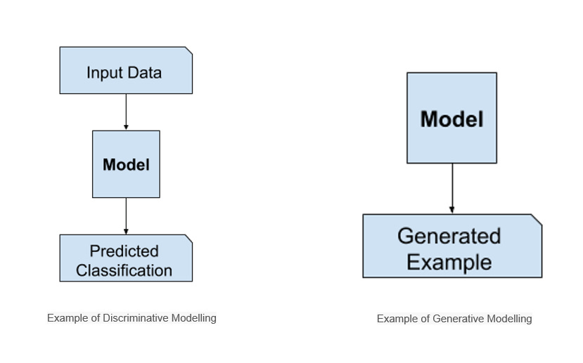
Image generation problem is where the machine learning model generates an image by itself. The set of images given for training and the model-generated image are similar to each other but not the same.

Here the issue is that we need a way to score the output image. If there are 2 output images, how can we say which one is better?

GAN (Generative Adversarial Networks) proposes to use a neural network for this process. So in addition to the model, there is another neural network that scores the image output. The neural net that generates the image is called Generator and the one that scores the image is called the Discriminator.

A Gentle Introduction to Generative Adversarial Networks (GANs) (machinelearningmastery.com)

GANs work great for multiple applications however, they are difficult to train, and their output lack diversity due to several challenges such as mode collapse and vanishing gradients to name a few.

To overcome this disadvantage, Diffusion Models came into being.

Diffusion Models are probabilistic likelihood estimation methods and take inspiration from physical phenomenon — thermodynamics of gas molecules whereby the molecules diffuse from high density to low density areas. In information theory, this equates to loss of information due to gradual intervention of noise.

Fundamentally, Diffusion Models work by destroying i.e. synthetic decay of training data through the successive addition of Gaussian noise, and then learning to recover the data by reversing this noising process — denoising.

More specifically, a Diffusion Model is a latent variable model which maps to the latent space using a fixed Markov chain. This chain gradually adds noise to the data in order to obtain the approximate posterior q(x1:T|x0), where x1,…,xT are the latent variables with the same dimensionality as x0. In the figure below, we see such a Markov chain manifested for image data.

Introduction to Diffusion Models for Machine Learning (assemblyai.com)

Ultimately, the image is asymptotically transformed to pure Gaussian noise. The goal of training a diffusion model is to learn the reverse process (denoising)— i.e. training pθ(xt−1|xt). By traversing backwards along this chain, we can generate new data.

MODEL: The diffusion process consists in taking random noise of the size of the desired output and pass it through the model several times. The process ends after a given number of steps, and the output image should represent a sample according to the training data distribution of the model, for instance an image of a butterfly. During training we show many samples of a given distribution, such as images of butterfly. After training, the model will be able to process random noise to generate similar butterfly images.

SCHEDULERS: It’s a library of diffusers that is used for the denoising process, a specific noise scheduling algorithm is thus necessary and “wrap” the model to define how many diffusion steps are needed for inference as well as how to compute a less noisy image from the model’s output.

PIPELINE: It groups together a model and a scheduler and make it easy for an end-user to run a full denoising loop process.

Code

First step is to Install Diffusers

!pip install diffusers==0.1.3

Import (Denoising Diffusion Probabilistic Model) DDPM Pipeline.

We’ll use the google/ddpm-celebahq-256 model, built in collaboration by Google and U.C. Berkeley. It's a model following the Denoising Diffusion Probabilistic Models (DDPM) algorithm trained on a dataset of celebrities images.

from diffusers import DDPMPipeline

The from_pretrained() method allows downloading the model and its configuration from the Hugging Face Hub, a repository of over 60,000 models shared by the community.

image_pipe = DDPMPipeline.from_pretrained("google/ddpm-celebahq-256")

The pipeline returns as output a dictionary with a generated sample of interest.

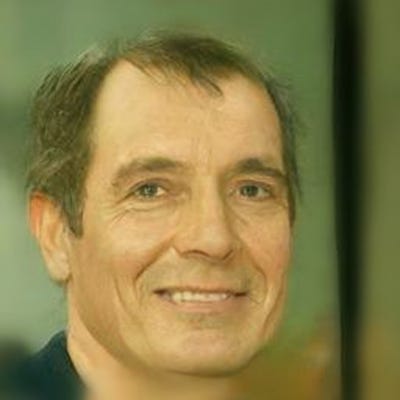
images = image_pipe()["sample"]

The image will be visible as:

images[0]

Models

from diffusers import UNet2DModelrepo_id = "google/ddpm-church-256"
model = UNet2DModel.from_pretrained(repo_id)

The from_pretrained() method caches the model weights locally, so if you execute the cell above a second time, it will go much faster.

import torch

torch.manual_seed(0)

noisy_sample = torch.randn(
    1, model.config.in_channels, model.config.sample_size, model.config.sample_size
)
noisy_sample.shape

The timestep is important to cue the model with “how noisy” the input image is (more noisy in the beginning of the process, less noisy at the end), so the model knows if it’s closer to the start or the end of the diffusion process.

with torch.no_grad():
    noisy_residual = model(sample=noisy_sample, timestep=2)["sample"]

Now, we'll check the shape of this noise residual

noisy_residual.shape

The predicted noisy_residual has the exact same shape as the input and we use it to compute a slightly less noised image. Let's confirm the output shapes match.

Schedulers

They define the noise schedule which is used to add noise to the model during training, and also define the algorithm to compute the slightly less noisy sample given the model output (here noisy_residual).

1. DDPM Scheduler:

from diffusers import DDPMScheduler

scheduler = DDPMScheduler.from_config(repo_id)

Now that the DDPM Scheduler is imported,

less_noisy_sample = scheduler.step(
    model_output=noisy_residual, timestep=2, sample=noisy_sample
)["prev_sample"]
less_noisy_sample.shape
import PIL.Image
import numpy as np

def display_sample(sample, i):
    image_processed = sample.cpu().permute(0, 2, 3, 1)
    image_processed = (image_processed + 1.0) * 127.5
    image_processed = image_processed.numpy().astype(np.uint8)

    image_pil = PIL.Image.fromarray(image_processed[0])
    display(f"Image at step {i}")
    display(image_pil)

Time to finally define the denoising loop

import tqdm

sample = noisy_sample

for i, t in enumerate(tqdm.tqdm(scheduler.timesteps)):
  # 1. predict noise residual
  with torch.no_grad():
      residual = model(sample, t)["sample"]

  # 2. compute less noisy image and set x_t -> x_t-1
  sample = scheduler.step(residual, t, sample)["prev_sample"]

  # 3. optionally look at image
  if (i + 1) % 50 == 0:
      display_sample(sample, i + 1)

While the quality of the image in DDPM is actually quite good — speed of image generation is slower.

2. DDIM Scheduler:

from diffusers import DDIMScheduler

scheduler = DDIMScheduler.from_config(repo_id)

The DDIM scheduler allows the user to define how many denoising steps should be run at inference via the set_timesteps method. The DDPM scheduler runs by default 1000 denoising steps. Let's significantly reduce this number to just 50 inference steps for DDIM.

scheduler.set_timesteps(num_inference_steps=50)

And you can run the same loop as before - only that you are now making use of the much faster DDIM scheduler.

import tqdm

sample = noisy_sample

for i, t in enumerate(tqdm.tqdm(scheduler.timesteps)):
  # 1. predict noise residual
  with torch.no_grad():
      residual = model(sample, t)["sample"]

  # 2. compute previous image and set x_t -> x_t-1
  sample = scheduler.step(residual, t, sample)["prev_sample"]

  # 3. optionally look at image
  if (i + 1) % 10 == 0:
      display_sample(sample, i + 1)

In DDIM, though the speed of image generation is faster, the quality of image is hindered.

So we can conclude schedulers as:

Subscribe to receive a copy of our newsletter directly delivered to your inbox.

The above article is sponsored by Vevesta.

Vevesta: Your Machine Learning Team’s Collective Wiki: Save and Share your Features and Techniques.

100 early birds who login to Vevesta will get free subscription for 3 months.

Machine Learning Diaries

Discussion about this post