DiffGrad : Is it the right optimization method for training your CNNs?
Learn about DiffGrad - optimizer that solves the overshooting problem of Adam
Background
Drawbacks of Stochastic Gradient Descent
The one of the basic approaches for finding an optimal solution while training neural networks is Stochastic Gradient Descent (SGD) optimization. Here, initially selected loss function is computed. Then, the gradient for each parameter (i.e., in each dimension) in the network is computed and the parameter values are updated in the opposite direction of the gradient by a factor proportional to the gradient. For SGD optimization, the above two steps are repeated until convergence or until a certain number of epochs or iterations are completed.
Following are the major drawbacks in the basic SGD approach:
1) If the loss changes quickly for a set of parameters and slowly for another set of parameters, then it leads to very slow learning along shallow dimensions and a jittering effect along steep dimensions.

2) If the loss function has a local minimum or a saddle point, then SGD gets stuck due to zero gradients in that region. Refer to Figure above.
3) The gradients are usually computed over minibatches; so, the gradients can be noisy.
4) SGD takes the same step for each parameter (i.e dimension) irrespective of the iteration-wise gradient behaviour for that parameter, which leads to poor optimization.
Sneak Peak on DiffGrad
The optimizer diffGrad uses the difference between the present and past gradients. It uses gradient behaviour to control the learning rate at the optimization stage resulting in an optimal solution. If the gradient difference is large this means that optimization is not stable and therefore the diffGrad allows a high learning rate. Conversely, if gradient difference is small, it means that model is close to an optimal solution. Then the diffGrad lowers the learning rate automatically [2].
DiffGrad Explained
In SGD the update is a dependent on previous value of the parameter, the learning rate at the t iteration and the gradient g at time t(which is differential of loss function w.r.t parameter theta.
Gradient descent methods such as AdaGrad, AdaDelta, RMSProp and Adam rely on the square roots of exponential moving averages of squared past gradients. Unlike DiffGrad, these methods do not take advantage of local change in gradients [1].
DiffGrad based on the difference between the present and the immediate past gradient. The step size is adjusted for each parameter in such a way that it should have a larger step size for faster gradient changing parameters and a lower step size for lower gradient changing parameters.
Evaluation of DiffGrad wrt other Optimizers
On comparing with other optimizers, it was observed that DiffGrad achieved the highest accuracy on batch sizes of 32, 64 and 128. It was trained and tested on a total data set of size 60000 images.

Comparision with Adam
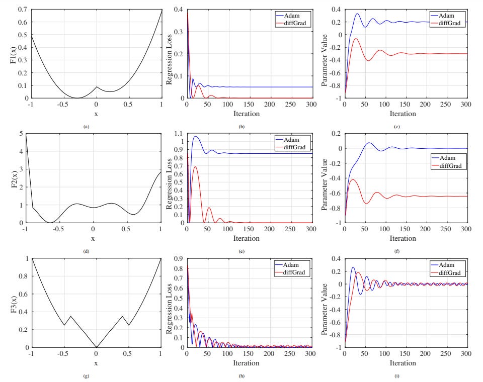
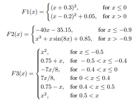
On multiple plots it can be seen that Adam overshoots global minima. In image F1(x), it can be seen from the plot (b) that Regression Loss using Adam stabilizes at around 0.6, while diffGrad is able to get the regression loss down to 0. Also, in parameter Value plot of F1(x), it can be seen that Adam overshoots the minima at -0.3 and stabilizes at parameter value 0.2 Similar behaviour of overshooting the global minima is observed in plots of F2(x).
Drawback of DiffGrad
The diffGrad uses fraction constant based on previous gradient information for gradient calculation. This fraction constant decreases the momentum resulting in slow convergence towards an optimal solution [2].


