How to use Cyclical Learning Rate to get quick convergence for your Neural Network?
Achieve higher accuracy for your machine learning model in lesser iterations.

The learning rate is a hyper-parameter that determines the pace at which an algorithm updates or learns the values of a parameter estimate. It regulates the amount of allocated error with which the model’s weights are updated each time they are updated, such as at the end of each batch of training instances.
If the learning rate used is low, the number of iterations/epochs required to minimize the cost function is high (takes longer time). If the learning rate is high, the cost function could saturate at a value higher than the minimum value. An optimal learning rate can cause our model to converge faster.

There are various sorts of learning rate approaches but here we will talk about Cyclical Learning Rate.
Cyclical Learning Rate is one of the approaches to achieve Optimal Learning Rates. The learning rate cyclically changes between a base minimum rate and a maximum rate in this methodology. The learning rate changes are cyclic, always returning to the learning rate's initial value.
A very high learning rate causes the model to fluctuate more or to diverge from the minima, while a lower learning rate can cause the model to converge very slowly or to converge to the local minima. Cyclical learning rate (CLR) allows keeping the learning rate high and low, causing the model not to diverge along with jumping from the local minima.
How Cyclic Learning Rate improves speed of convergence?
In CLR, we vary the Learning Rates between a lower and higher threshold. In other words, learning rate oscillates between base (minimum) learning rate and maximum learning rate. This helps as follows:
Periodic higher learning rates within each epoch helps to come out of any saddle points or local minima if it encounters into one. Saddle points have small gradients that slow the learning process.
According to authors, when using CLR it is likely the optimum learning rate will be between the bounds and near optimal learning rates will be used throughout training.
In the figure below, Classification accuracy has been plotted with multiple learning rates while training on CIFAR-10. The red curve shows the result of training with one of the CLR (Cyclic Learning rate) policy. The implication is clear: The baseline (blue curve) reaches a final accuracy of 81.4 % after 70, 000 iterations. In contrast, with CLR, it is possible to fully train the network (red curve) within 25,000 iterations and attain the same accuracy.
Types of Cyclic Learning Rates
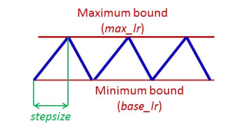
At a constant frequency, the learning rate varies in a triangular pattern between the maximum and base rates. The oscillation of learning rate can be based on various function-triangular (linear), Welch window (parabolic), or Hann window (sinusoidal).
The Triangular Window
The triangular window is a simpler way of changing the learning rate that is linearly increasing with some constant from min learning rate to max learning rate then linearly decreasing with the same constant from max learning rate to minimum learning rate.

The idea is to divide the training process into cycles determined by a stepsize parameter. This code varies the learning rate linearly between the minimum (base LR) and the maximum (max LR)
LR: the computed learning rate
opt.LR: the specified lower (base) learning rate
maxLR: Maximum learning rate boundary
epochCounter: the number of epochs of training
cycle length: Number of iterations until the learning rate returns to the initial value.
stepsize: the number of iterations in half a cycle
Implementation Nuggets
According to authors, following needs to be kept in mind while training with CLR:
stepsize should be equal to 2–10 times the number of iterations in an epoch. We can calculate iterations present in an epoch using dataset size and batch size. If the dataset comprises 50,000 data entries and the batch size is 100, then the number of iterations in an epoch will be 500 (50,000/100).
Experiments show that replacing each step of a constant learning rate with at least 3 cycles trains the network weights most of the way and running for 4 or more cycles will achieve even better performance.
Also, it is best to stop training at the end of a cycle, which is when the learning rate is at the minimum value and the accuracy peaks.
Set base learning rate (or opt.LR) to 1/3 or 1/4 of maximum learning rate. Alternatively, run the model for few epochs when given a new architecture or dataset. Plot learning rate and accuracy as shown in the figure below. Note the learning rate value when the accuracy starts to increase, set this learning rate as base learning rate. And when the accuracy drops or slows or becomes ragged, set it to maximum learning rate. Example: from the plot, it can be seen that we can set base lr = 0.001 because the model starts converging right away. Furthermore, above a learning rate of 0.006 the accuracy rise gets rough and eventually begins to drop so it is reasonable to set max lr = 0.006.
Conclusion:
Only a few epochs where the learning rate linearly increases is sufficient to estimate boundary learning rates for CLR.
Use of cyclic functions as a learning rate policy leads to substantial improvements in performance for a range of architectures.
The cyclic nature of CLR guides when to drop the learning rate values (after 3 - 5 cycles) and when to stop the training.
Subscribe to receive a copy of our newsletter directly delivered to your inbox.
The above article is sponsored by Vevesta.
Vevesta: Your Machine Learning Team’s Feature and Technique Dictionary - Accelerate your Machine learning project by using features, techniques and projects used by your peers
100 early birds who login into Vevesta will get free lifetime access to the tool
References:
This article was originally published at https://www.vevesta.com/blog/31-Cyclical-Learning-Rates


