Beginner’s Guide to DBSCAN Clustering
Unsupervised clustering technique for arbitrary shaped clusters
Clustering is the technique of dividing a population or set of data points into groups so that data points in the same group are more similar to data points in other groups than data points in other groups. In other words, the goal is to separate groups with similar characteristics and assign them to clusters.
There is no label attached to the data points because it is an unsupervised learning method. The algorithm attempts to discover the data’s underlying structure. K-Means (distance between points), Affinity propagation (graph distance), Mean-shift (distance between points), DBSCAN (distance between nearest points), Gaussian mixtures, and other methods are included.
Let’s get started with a detailed examination of the DB Scan Algorithm in this article.
With normal shaped clusters, partition-based or hierarchical clustering techniques are highly efficient. However, density-based techniques are more efficient when it comes to detecting outliers or arbitrary shaped clusters.
Consider the following graphs.
These figures’ data points are organised in arbitrary shapes or contains outliers. When compared to Normal K-Means or Hierarchical Clustering Algorithms, density-based clustering algorithms are much more efficient at finding high-density regions and outliers.
DBSCAN
Density-Based Spatial Clustering of Applications with Noise is the acronym for the DBSCAN algorithm. It can find arbitrary-shaped clusters as well as clusters containing noise (i.e. outliers).
The DBSCAN Algorithm is based on the premise that a point belongs to a cluster if it is close to numerous other points in that cluster.
There are two key parameters of DBSCAN:
eps(Epsilon): The distance that defines the neighborhoods. Two points are considered to be neighbors if the distance between them is less than or equal to eps.
minPts(minPoints): Minimum number of data points that are required to define a cluster.
Based on these two parameters, points are classified as core point, border point, or outlier:
Core point: A point is said to be a core point if there are at least minPts number of points (including the point itself) in its surrounding area with radius eps.
Border point: A point is a border point if it is reachable from a core point and there are less than minPts number of points within its surrounding area.
Outlier: A point is an outlier if it is not a core point and not reachable from any core points.
The following figure is taken from researchgate.net.
How does the DBSCAN Algorithm create Clusters?
The DBSCAN algorithm begins by randomly selecting a point (one record) x from the dataset and assigning it to cluster 1. Then it counts how many points are within (epsilon) distance of x. If this quantity is larger than or equal to minPoints (n), it is considered a core point, and all these -neighbors are pulled into the same cluster 1. It will next look at each member of Cluster 1 and find their -neighbors. If any member of cluster 1 has n or more -neighbors, it will enlarge the cluster by adding those -neighbors. Cluster 1 will be expanded until there are no more data points to put in it.
In the latter instance, it will select another point from the dataset that does not belong to any of the clusters and assign it to cluster 2. This will continue until all data points either belong to a cluster or are designated as outliers.
DBSCAN Parameter Selection
DBSCAN is extremely sensitive to the values of epsilon and minPoints. A slight variation in these values can significantly change the results produced by the DBSCAN algorithm. Therefore, it is important to understand how to select the values of epsilon and minPoints.
minPoints(n):
As a starting point, a minimum n can be derived from the number of dimensions D in the data set, as n ≥ D + 1. For data sets with noise, larger values are usually better and will yield more significant clusters. Hence, n = 2·D can be a suggested valued, however this is not a hard and fast rule and should be checked for multiple values of n.
Epsilon(ε):
If a small epsilon is chosen, a large part of the data will not be clustered whereas, for a too high value of ε, clusters will merge and the majority of objects will be in the same cluster. Hence, the value for ε can then be chosen by using a k-graph. Good values of ε are where this plot shows an “elbow”.
Code
Importing the Libraries
import numpy as np
import pandas as pd
from sklearn.datasets import make_blobs
from sklearn.preprocessing import StandardScaler
import matplotlib.pyplot as plt
%matplotlib inline
Generating Clustered Data From Sklearn
X, y = make_blobs(n_samples=1000,cluster_std=0.5, random_state=0)plt.figure(figsize=(8,6))
plt.scatter(X[:,0], X[:,1], c=y)
plt.show()
Initialization and Fitting the model.
from sklearn.cluster import DBSCAN
db = DBSCAN(eps=0.4, min_samples=20)
db.fit(X)
y_pred = db.fit_predict(X)
Plotting the clustered data points
plt.figure(figsize=(8,6))
plt.scatter(X[:,0], X[:,1],c=y_pred)
plt.title("Clusters determined by DBSCAN")
plt.show()
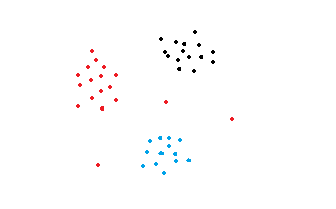
Although the clusters in this sample dataset do not have arbitrary shapes, we can see that DBSCAN fared exceptionally well at spotting outliers, which would be difficult with partition-based (e.g., k-means) or hierarchical (e.g., agglomerative) clustering approaches. DBSCAN would still outperform the other two clustering techniques listed above if we applied it to a dataset with arbitrarily shaped clusters.
Credits
The above article is sponsored by Vevesta.
Vevesta: Your Machine Learning Team’s Collective Wiki: Identify and use relevant machine learning projects, features and techniques
For more such stories, follow us on twitter at @vevesta1
100 early birds who login to Vevesta get free subscription for 3 months.
References
Subscribe to our weekly newsletter to stay updated on latest machine learning/MLOps articles.


